wtd-dsl
Design and Implementation of Wind Tunnel Deisgn Domain Specific Language: pipeflow
Working process with backward!
- write for press conference
- write manual
- write requirements
- write test suites
- write libraries
- write GUI
Press Conference
Here we proudly anounce a DSL for wind tunnel aerodynamic design, pipeflow.
It represents excellent aerodyanmic deisgn of wind tunnels as compilable & runnable program! It enables systematically exploring design space of wind tunnels. It boosts robustness and edgeness of next generation wind tunnel design.
Wind tunnel design to run! Wind tunnel design to git! Wind tunnel design to reuse!
Domain analysis
Wind tunnel design results are geometric definitions fo a tunnel circuit, where wind tunnel components are defined, the geometric parameters are specified for each components, the connection relationship between components is defined. For all the operational conditions, the performance of the tunnel circuit and components will be prodicted to specified design requirements of the fan/compressor. At some point, the fan map wille be presented as the start point to design the fan. At the first design phase, the aerodynamic design of the fan will not be included.
operational conditions & operational envolop
geometry
Wind tunnel components are very simple things, they are just pipes, with inlet (inflow intersection), outlet (outflow intersection), profile (a series of intersections along its length).
\[\mathcal{S}_i = \mathcal{S}_i(r), ~\mathrm{for}~ r \in [0, L_i]\]where $\mathcal{S}_i(r)$ is a simply-connected 2D area ($\Omega$) by closed curve ($\partial \Omega$) in $xy$-plane.
Perimeter and area are as follows: \(C = \int_{\partial\Omega} ds\) where $s$ denotes the arc length on the curve $\partial\Omega$, starting and ending at any arbitrary point on $\partial\Omega$.
\(A = \int_\Omega dxdy\) Hydraulic diameter will be: \(D = \frac{4A}{C}\)
For any intersection, a two dimensional shape can be defined as the flow area, usually circle, rectangle, square, or octagon (often referred as cutted rectangle). For the concern of wind tunnel design, the area of the shape, the hydraulic diameter are the two things that matter.
Only when we consider the pressure loss of pipe component, actual shape of intersection do matters, where a shape coefficient can be defined to express anomolic feature that the shape can affect energy loss when flow through the intersection.
Pressure loss and other performance indexes
For any component, under the constaint that there is no separation in it, the pressure loss coefficient (local or reduced by nomolization of testsection dynamic pressure) is the primary design drive. For setting chamber, contraction (\& plus nozzle), and testsections, there are also uniformity indexes. There are noise performance for specific types of wind tunnels. Nevertheless, pressure loss is the primary performance loss for almost all components in windtunnel circuit.
Taking construction in mind, the aerodynamic design also partially determines the construction cost of a wind tunnel. And pressure losses are essential to derive windtunnel fan map, which determines the most expensive component in the sense of runtime cost of windtunnel experiments.
graph TD
A(Total cost) --> C(Continuous runtime cost)
A --> B(One-time construction cost)
B --> E
C -----> KK[[Experiments design]]
C --> E(Fan/Compressor operation map) --> F[Pressure loss of components] --> D
B ----> D(Components geometric parameters) --> AP[[Aerodynamic design]]
PI(Performance) ---> PIA(Operational envolop) --> F
PI --> PIB(FLow Uniformity in testsection) ---> D
PI ---> xx(Efficiency)----> ef[[Process design]]
PC(Performance/cost ratio) --> A
PC --> PI
graph TD
A(成本) --> C(运行成本)
A --> B(建设成本)
B --> E
C -----> KK[[试验设计]]
C --> E(风扇图谱) --> F[部段损失] --> D
B ----> D(回路几何) --> AP[[气动设计]]
PI(性能) ---> PIA(运行包线) --> F
PI --> PIB(流场品质) ---> D
PI ---> xx(试验效率)----> ef[[过程设计]]
PC(效费比) --> A
PC --> PI
As Fig. 1 describes, the aerodynamic design represents as components in the circuit and geometric parameters defined. From circuit laytouts and parameters of components, mechanmical engineers can estimate the one-time construction cost; aerodynamists can estimate the pressure loss of all components and flow uniformity in the test section. From pressure loss, aerodynamists can estimate the operational envolop ot the tunnel, and design fan map. The latter leads to continuous runtime cost of the tunnel, combined with experiments design. While operational envolop and flow quality consists the performance of a wind tunnel, one-time construction cost and continuous runtime cost consists the total cost of the tunnel.
fan map
But fan map must be specified with the design of the circuit.
For low-speed windtunnel fan, the driving pressure produced is expressed as $\Delta P=P_1-P_0$, for high-speed windtunnel compressor, the pressure is expressed as pressure ratio $\xi = P_1/P_0$ \(\Delta P = f(\dot{m}, P_0, T_0, N_\textrm{rpm}, v_0, \ldots) \\ \xi = f(\dot{m}, P_0, T_0, N_\textrm{rpm}, v_0, \ldots)\) This is one of the main production of aerodynamic design.
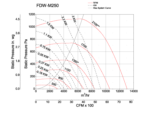
Usually, the fan map is series of $\Delta P ~\mathrm{v.s.}~ \dot{m}$ for different parameter combinations. As Fig.2 shows, a series of red curves show the operational parameters with predefined roational speed (RPM). The solid black curve is the maximum pressure points with given RPMs. Usually, this will be the design curve of the wind tunnel. And a series of dashed curves show the $\Delta P ~\mathrm{v.s.}~ \dot{m}$ relationship with given power input. This performance map contains all the information needed to carry out aerodynamic design.
For wind tunnels, fan work on flow can be expressed as a function of mass flow rate and pressure rise: \(\begin{array}{ll} W&= Q \cdot \Delta P \\ &= \rho_t v_t A_t \cdot \varepsilon_T \frac{1}{2} \rho_t v_t^2 \\ &= \frac{1}{2} \rho_t^2 v_t^3 A_t \varepsilon_T \\ &= \frac{1}{2} \rho_t^2 \left(\frac{Q}{\rho_t A_t}\right)^3A_t\varepsilon_T \\ &= \frac{1}{2} \frac{\varepsilon_T}{\rho_t^2 A_t^2} Q^3 \end{array}\)
\[\begin{array}{ll} \Delta P &= \varepsilon_T \frac{1}{2} \rho_t v_t^2 \\ &=0.5\varepsilon_T \rho_t \frac{Q^2}{\rho_t^2 A_t^2}\\ &=\varepsilon_T \frac{1}{2\rho_t A_t^2} Q^2 \end{array}\]Total pressure loss coefficient $\varepsilon_T$, density and velocity in the test section define designed curve in the fan map.
loss coefficients
And $\varepsilon_i$ to normalize loss $\hat{\varepsilon}_i$ . \(\varepsilon_i = \frac{\Delta P_i}{\frac{1}{2}\rho v^2}\) Normalized loss coefficients are normalized by dynamic pressure at the test section: \(\hat{\varepsilon}_i = \frac{\Delta P_i}{\frac{1}{2}\rho_tv_t^2}\) By continuous equation: \(\rho_i v_i A_i = \rho_t v_t A_t\) For the whole circuit, the loss coefficients is: \(\varepsilon_T = \sum_i{\hat{\varepsilon_i}}\)
Total pressure loss is \(\Delta P_T = \frac{1}{2}\rho_tv_t^2 \cdot \varepsilon_T\)
DSL abstract design and concrete design
syntax
The syntax for describes a wind tunnel aerodynamic design consists of several different parts.
- wind tunnel definitions
- components geometric definitions
- connection relationship definitions
- profile definitions
- intersection definitions
- Operational definitions
- operational envolop
- design points definitions
- experiments frequencies
- Performance definitions
- component pressure loss
- test section flow uniformity
- fan map generation
- components geometric definitions
Design
- All entities (Windtunnel, components, profile, intersection) are identified by string names.
- Descriptive vocabularies are used to record the design of entities.
- Mathematical declarations of geometries are used with definition of numerical variables.
- Unique formal declarations can be generated for comparisons and storages.
- Performance indexes can be generated for geometrical description.
- Variables are sweepable.
- Variables are optimizable.
Entity hierarchy
graph TD
A(Wind tunnel) --- B(Component)
B --- C(Profile) --- D(Intersection) --- E(Variable)
variable name "tsl" length meter
variable name "d" length meter
variable name "vts" velocity mps
variable name "p0" pressure pa
variable name "rho0" density kgpmc

windtunnel name "0.3mx0.3m low speed teaching wind tunnel" shorthand "0.3m lstwt"
windtunnel name "0.3m lstwt" cc "0.3m test section" shorthand "ts#1"
cc name "ts#1" length varialbe name "tsl"
cc name "ts#1" profile {
    rectangle width 0.3 height 0.4
}
windtunnel name "0.3m lstwt" cc "diffuser #1"
cc name "diffuser #1" length 6.0.meters
cc name "diffuser #1" profile {
    rectangle width 0.3 height 0.4 + 0.1 * it / 6.0
}

cc name "ts#1" + cc name "diffuser #1"
classDiagram

class WindTunnelCircuit {
    +List~CircutComponent~ components
    +bool isCloseLoop
    +String name
    +totalLossCoefficient() Double
    +upstream(c: CircutComponent) CircutComponent
    +downstream(c: CircutComponent) CircutComponent
    +testsection() TestSection
}
classDiagram
class CircuitComponent{
    +String name
    -CircutComponent upstream
    -CircutComponent downstream
    +Profile profile
    +localLossCoefficient(massflowrate: Double) Double
}
CircuitComponent <|-- TestSection
CircuitComponent <|-- Diffuser
CircuitComponent <|-- Corner
CircuitComponent <|-- Backleg
CircuitComponent <|-- HeatExchanger
CircuitComponent <|-- Fan
CircuitComponent <|-- SettlingChamber
CircuitComponent <|-- Contraction
CircuitComponent <|-- SecondThroat
CircuitComponent <|-- Reentry
classDiagram
class Profile{
    +String name
    +Variable length
    +intersection(x: Double) Shape
}
Profile <|-- LinearProfile
Profile <|-- CurveProfile
Profile <|-- TransitionProfile
classDiagram

Shape <|-- Circle
Rectangle <|-- Square
Shape <|-- CuttedRectangle
CuttedRectangle <|-- Rectangle
Shape <|-- RectangleCircleTransitSection
class Shape {
    +Variable hydraulicDiameter
    +perimeter()* Double
    +area()* Double
}
class RectangleCircleTransitSection{
    +Double radius
    +Double cutSquareSide
    +perimeter() Double
    +area() Double
}
class Circle {
    +Double radius
    +perimeter() Double
    +area() Double
}
class CuttedRectangle {
    +Double weight
    +Double height
    +Double cw
    +Double ch
    +perimeter() Double
    +area() Double
}
class Rectangle {
    +CuttedRectangle(weight, height, 0, 0)
}
class Square{
    +Rectangle(d, d)
}
classDiagram
class Variable{
    +String name
    +Double lb
    +Double ub
    +Double value
    +sweep(lb:Double, ub:Double, n:Integer)
}
semantics
Kotlin toolbox for DSL implementation
How Kotlin utilities help to implement a DSL will definitely affect the way we design the DSL.
- Exploit the power of Kotlin to create fluent code
- Extend the vocabulary of the APIs bring in domain-specific code
- Program implicit context so the DSLs are concise and easy to work with
- Manage the scope of calls and handle errors gracefully
Exploit Fluency
object fetch {
    infix fun balance(number: Int) = println("Fetch the balance for $number")
}
This code make fetch balance 12345 legitimate code.
Implementing infix functions with more than two arguments.
enum class Message {
    StatementReady,
    LowBalanceAlert;

    infix fun to(number: Int) = println("sending message $this to $number")
}

object send {
    infix fun message(messageId: Message) = messageId
}

send message StatementReady to 123456
Make programming easier with plain grammar like this:
account number 123455 withdraw 1000
account number 12345 deposit 1000
The benifits of using Kotlin to implement the above syntax are: 1) the script or program will contain minimum extra programming flavor to let domain engineers write code more comfortablelly and confidently, 2) the above natural language script is totally legitimate Kotlin code, so current full-feature IDE can or LSP can be used to check the validity of DSL program.
function as parameter and syntax sugar
First check with and apply in kotlin stdlib.
public inline fun <T, R> with(receiver: T, block: T.() -> R): R{
    contract{
        callsInPlace(block, InvocationKind.EXACTLY_ONCE)
    }
    return receiver.block()
}
public inline fun<T> T.apply(block: T.()->Unit): T {
    contract{
        callsInPlace(block, InvocationKind.EXACTLY_ONCE)
    }
    block()
    return this
}
extension function
operator overload
infix function
Other facilities
User Manual
Define design
Define wind tunnel aerodynamic design with kotlin as follows:
windtunnel("0.5m teaching wind tunnel") {
    testsection("#1")  {
        length = 3.0
        profile {

        }
    }

    diffuser("#1 diffuser") {}

    fan("#fan") {}

    diffuser("#2 diffuser") {}

    collector("#collector") {}

    settlingchamber("#sc") {}

    contraction("#ctr") {}

    openCircuit("# collector", "#sc", "#ctr", "#1", "#1 diffuser", "#fan", "#2 diffuser")
}
Evaluate performance
For database, load performance data, and predict the performance of current design.
Developer Manual
Requirements
Test suites
Libraries
UI/UX development
References
- Bin Ali, Hussain & mahesh, Ramagiri & kishore, M & shabaaz, Md. (2020). DESIGN AND DRAFTING OF AIR CONDITIONING SYSTEM FOR A RESIDENTIAL BUILDING USING AIR COOLED CHILLERS. 10.13140/RG.2.2.20434.99528.